The Collatz Conjecture is one of the most famous unsolved problems in mathematics. It proposes a simple algorithm: take any positive integer and repeatedly apply these rules:
- If the number is even: divide it by 2
- If the number is odd: multiply it by 3 and add 1
The conjecture states that no matter which number you start with, you will always eventually reach the number 1 and then cycle 1 → 4 → 2 → 1 indefinitely. This has been verified for trillions of numbers, but no proof exists yet!
Example: Drawing a trajectory from a sample
Take sample number, say 9, and apply the Collatz alpgorithm:
This sequence of 19 steps is called the trajectory. The number 1 is the root (the minimum value in the cycle 4-2-1).
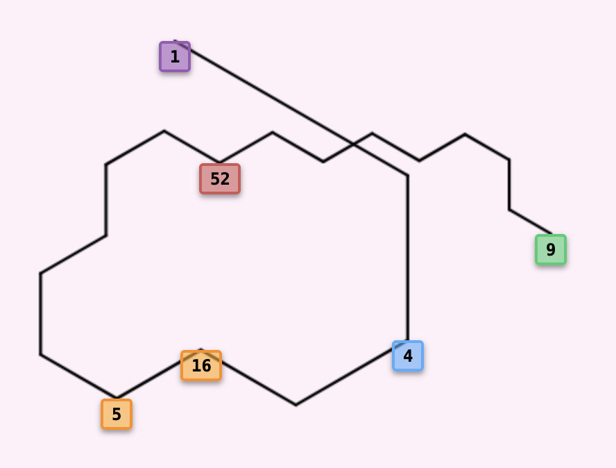
→ 10 → 20 → 40 → 13 → 26
→ 52 → 17 → 34 → 11 → 22
→ 7 → 14 → 28 → 9
- ➜ 60° Clockwise: If next number is even
- ➜ 60° Counterclockwise: If next number is odd
Starting horizontally, the line makes a 60° turn at each step: turning clockwise towards an even number, and counterclockwise towards an odd number. The resulting jagged pattern beautifully reveals the rhythm and structure hidden within the sequence, with alternating turns creating the distinctive zigzag pattern. This visual representation makes it immediately apparent which numbers are even and which are odd throughout the entire sequence.
Example: An Alternative Collatz conjecture
This visualizer also supports alternative rules. For instance:
- If even: divide by 2, then add 1
- If odd: multiply by 3 and add 1 (same as classic)
Notice that the root here is 21 (the minimum in the cycle), not 5 (the minimum of the sequence) or 40 (the start of the cycle)!
But for this set of rules, there is more than one outcome. For example, starting from another sample we end up in a different cycle.
And even a boring case of a single number 2 that goes to itself and nothing else converges to it.
Different Number of Rules
You can even define sequences based on remainders modulo 3:
- If n % 3 = 0: divide by 3
- If n % 3 = 1: multiply by 2 and add 1
- If n % 3 = 2: multiply by 4 and add 2
Possible cycling sequences would be
The beauty of this visualizer is that it works with any modulus and any rules you define! If in your rule set the sample value diverges to infinity or does not converge for too long, the script will skip this value.
Understanding the Tree Visualization
▼Instead of showing single sequences, the visualizer builds trees. Here's how:
- You choose a range of starting numbers (e.g., from 1 to 100)
- For each number, trace its Collatz sequence until it reaches a cycle
- All sequences that reach the same cycle form a tree with the cycle's minimum as the root
- Branches show which numbers lead to which other numbers
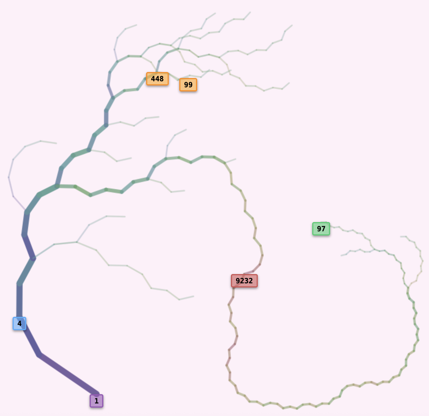
- ● 1 (Purple): Root node
- ● 4 (Blue): Cycle start (where the root points to)
- ● 97 (Green): Deepest leaf
- ● 9232 (Red): Highest value
- ● 99 (Orange): Start value (chosen to be the last from the sample)
- ● 448 (Orange): Max height from 99
-
Branch angles:
- ● 28° to even nodes
- ● -49° to odd nodes
The sequence from the deepest leaf, 97, passes through the highest value, 9232, on its way down to the root at 1 and loops to the cycle 1→4→2→1...
Example Node Metrics
Here are the key metrics (weight, height, depth) for several nodes in a classic Collatz tree with values below 100 (see the figure above):
| Metric | Definition | Node 52 | Node 53 | Node 97 | Node 98 | Node 99 |
|---|---|---|---|---|---|---|
| Weight | Number of leaves that pass through this node | 10 | 6 | 1 | 1 | 1 |
| Height | Maximum value encountered on path to root | 52 | 160 | 9232 | 148 | 448 |
| Depth | Number of steps to reach root | 11 | 11 | 118 | 25 | 25 |
Branch Thickness (Weight Encoding)
Branch thickness encodes the weight of each node. Thicker branches indicate more leaves have their path to the root through them. Thinner, more transparent branches represent rare or specialized paths.
The line thickness uses is proportional to 2+log2(weight), which scales dynamically with the number of leaves.
This logarithmic encoding is optimal because each node can potentially split the weight in half.
The tree above has only 19 leaves in total, and 16 of them treminate via 40 → 20 → 10 → 5 → 16 → 8 → 4 → 2 → 1,
so the node 40 has weight 16, then it splits into a branch of weight 10 (40 ← 13 ← 26 ← 52) coming from the direction of 99, and a branch of weight 6 (80 ← 160 ← 53) coming from the direction of 97.
Branch Length (Depth Encoding)
As nodes get deeper in the tree (further from root), their branches become progressively shorter. This prevents deep trees from sprawling infinitely across the canvas while still maintaining visual clarity at multiple depths. The branch length follows a inverse square root relationship provides optimal scaling. Tt compresses rapidly at shallow depths but gradually for deeper nodes.
Branch Colors (Value Encoding)
Each branch's color represents the logarithm of the child node's numerical value. The entire spectrum from purple-blue (small numbers) through cyan, green, yellow, to red-orange (large numbers) is generated dynamically, the largest value branch in the tree is always red. Here's a continuous gradient showing how node values map to hues:
(Purple-Blue)
(Cyan-Green-Yellow)
(Red-Orange)
Special Node Highlights
Certain important nodes are marked with colored boxes:
Root (Purple)
The minimum cycle value. The foundation of the tree.
Cycle Start (Blue)
Where the root points to in the cycle.
Deepest Node (Green)
The node furthest from the root (longest path).
Highest Node (Red)
The node with the largest numerical value.
Smallest Node (Yellow)
The node with the smallest numerical value.
Highlighted (Orange)
The currently selected start value.
Interacting with the Tree
▼Define the sample set
Number of Samples
How many starting numbers to test. More samples = more detail but slower.
Lower Limit
Only consider starting samples above this number. Default: 1
Range
The span of numbers to consider (upper limit = lower + range). If the range is smaller than the number of samples, then every number from the range is sampled.
Select the tree
Select Tree
Choose which tree to display (populated after clicking "Build Trees"). Different cycles create diferent trees.
Start Value
Enter any number to pick the root to which this value converges to. If it has not been considered before, it will be added to the corresponding tree and processed correctly and the wights will be recomputed. The start value and its height will be highlighted in the tree.
By default the tree containing the start value is rendered, but you can lock the tree selection by the root, and start values from different trees will not cause them to be rendered. This helps when you are trying to populate a tree that only coveres a small fraction of samples.
Define rules
Modulus (Number of rules)
The number of different rules. Each rule applies based on the remainder modulo this number. Change this and new rule input fields appear automatically.
Individual Rules
For each remainder, set a formula to compute the next number in the sequence. This will determine the structure of the tree. For example, if Modulus = 2, you will have have rules for "n % 2 = 0" (even) and "n % 2 = 1" (odd). Each rule is a JavaScript expression: n/2, 3*n+1, etc.
Configure angles
Initial Angle
The starting direction for the root's branches (default: 0° is upwards). Range: -180° to +180°.
Branch Angles
For each rule, set the angle offset. Adjust branch angles precisely to 0.1° This determines how branches spread out from their parents. Adjust angles to create visually pleasing tree layouts. Angles update in real-time!
Other buttons and toggles
Build Trees
Reads all your settings and constructs the tree(s). This can take a few seconds for large samples.
Load Trees
Load a tree from a json file (the one you get after pressing "Save Tree Data"). Alternatively you can pick from a list of pre-existing trees to get some inspiration!
Hide/Show Labels
Toggle the colored node labels (special nodes highlighted with boxes).
Dark/Light Background
Switch between dark and light canvas backgrounds for better visibility or preferred aesthetics! 🌓
Download Image
Export the current tree as a high-resolution PNG image (4000px+) respecting your label and background settings.
Download Tree Data
Export the current configurateion (rules, angles) and leaves of the current tree as a json file. It can be shared or later uploaded in Load Tree. Only the current tree is saved, the other roots are ginored
Fit to Screen
Automatically zoom and pan to fit the entire tree in the screen.
Interactive canvas
- Zoom: Scroll up/down with your mouse wheel
- Pan: Click and drag the tree to move it around
- Auto-fit: Click the "Fit to Screen" button to see the entire tree
Hover over any node to see a tooltip showing its Value, Weight, Depth and Height
Click on any node to set it as your "Start Value". The tree will automatically update to highlight this node and its height.
Frequently Asked Questions
▼Is this the Collatz Tree Visualizer?
Yes, it is.
Can I visualize different Collatz trees with this tool?
Yes, you can.